Reliability block diagram calculation: a 1,000-hour series-parallel example

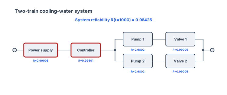
For this two-train cooling-water example, the calculated probability of completing a 1,000-hour mission without a modeled failure is 0.984251, or 98.4251%. The parallel pump trains alone reach 99.9127%, but the shared power supply and controller remain in series. Their combined reliability limits the whole system and makes both shared blocks single points of failure.

Scope: reliability over one mission, not availability

A reliability block diagram (RBD) asks which component functions must succeed for the system function to succeed. A series connection means every connected function is required. A parallel connection means any complete path is sufficient. IEC 61078:2016 covers using RBDs for qualitative and quantitative dependability analysis, including constant and time-dependent block probabilities; this example uses only a simple, non-repaired series-parallel model.

Here, reliability R(t) is a dimensionless probability evaluated at mission time t. It is not availability. Availability can include repair and restoration during the observation period; this calculation stops at the first modeled failure and includes no repair process.

The fictional system must provide cooling water continuously for 1,000 h. One shared power supply and one shared controller are required. Downstream, either of two active trains can meet demand, but a train succeeds only when both its pump and isolation valve succeed.

Inputs and assumptions

Block	Quantity supplied	Mission model	R(1,000 h)
Power supply	MTBF = 100,000 h	Exponential, constant hazard	0.9900498
Controller	MTBF = 200,000 h	Exponential, constant hazard	0.9950125
Pump 1 and Pump 2	MTBF = 50,000 h each	Identical, independent	0.9801987 each
Valve 1 and Valve 2	MTBF = 100,000 h each	Identical, independent	0.9900498 each
Mission time	1,000 h	No repair during mission	—

The worked result assumes statistically independent block failures, identical duties for the two trains, successful detection and use of the surviving train, and no capacity derating. The MTBF inputs are illustrative engineering data, not field estimates for a real product.

The NIST/SEMATECH e-Handbook gives the exponential reliability function as:

R(t) = e^(-lambda × t)
lambda = 1 / MTBF
therefore R(t) = e^(-t / MTBF)

The units must cancel. With t and MTBF both expressed in hours, t / MTBF is dimensionless and can be used as the exponential’s argument. Mixing hours with years or interpreting an MTBF as a guaranteed service life would invalidate the calculation.

Reproducible Schematex source

rbd "Two-train cooling-water system"
  mission: 1000
  series {
    block PSU "Power supply" mtbf=100000
    block CTRL "Controller" mtbf=200000
    parallel {
      series {
        block P1 "Pump 1" mtbf=50000
        block V1 "Valve 1" mtbf=100000
      }
      series {
        block P2 "Pump 2" mtbf=50000
        block V2 "Valve 2" mtbf=100000
      }
    }
  }

This source was validated and rendered with Schematex 1.0.9 on August 13, 2026. The current RBD syntax reference documents series, parallel, kofn, constant R, failure probability p, MTBF, failure-rate, and Weibull inputs. The owned documentation establishes renderer capability; the IEC and NIST sources listed below establish the dependability scope and equations.

Step 1: convert each MTBF to mission reliability

For the power supply:

R_PSU(1,000 h) = e^(-(1,000 h) / (100,000 h))
               = e^(-0.01)
               = 0.9900498

The remaining component values follow the same calculation:

R_CTRL = e^(-(1,000 h) / (200,000 h)) = 0.9950125
R_PUMP = e^(-(1,000 h) /  (50,000 h)) = 0.9801987
R_VALVE = e^(-(1,000 h) / (100,000 h)) = 0.9900498

These probabilities apply only to the stated 1,000-hour mission and the constant-hazard assumption. MTBF does not mean that a component will survive for its MTBF duration, and it does not describe infant mortality or wear-out behavior.

Step 2: reduce each series train

NIST’s series model multiplies independent component reliabilities because every component in the path must survive. Each pump train therefore has:

R_TRAIN = R_PUMP × R_VALVE
        = 0.9801987 × 0.9900498
        = 0.9704455

A useful invariant appears immediately: a series result cannot exceed the reliability of its least reliable component. 0.9704455 is below both 0.9801987 and 0.9900498, so the direction of the calculation is plausible.

Step 3: combine the two active-parallel trains

For two independent active-parallel paths, the subsystem fails only when both complete trains fail. NIST expresses that rule by multiplying the component failure probabilities and subtracting from one:

R_PARALLEL = 1 - (1 - R_TRAIN1)(1 - R_TRAIN2)
           = 1 - (1 - 0.9704455)^2
           = 1 - 0.0295545^2
           = 0.9991265

The parallel result must be at least as high as either branch reliability. Here it rises from 0.9704455 per train to 0.9991265 for the redundant subsystem. That gain depends on independence and on both trains being genuinely capable of the full required function.

Step 4: restore the shared series blocks

The power supply, controller, and equivalent parallel subsystem are all required, so their reliabilities multiply:

R_SYSTEM = R_PSU × R_CTRL × R_PARALLEL
         = 0.9900498 × 0.9950125 × 0.9991265
         = 0.9842515

Rounded to six decimal places, the result is 0.984251, or 98.4251%. Its complement is the modeled mission unreliability:

Q_SYSTEM = 1 - R_SYSTEM
         = 1 - 0.9842515
         = 0.0157485
         = 1.57485%

Across 1,000 statistically identical missions, that probability corresponds to an expectation of about 15.75 unsuccessful missions. It is not a rate of 15.75 failures per 1,000 h; the model result is a per-mission probability.

Structural checks before trusting the number

The arithmetic and the diagram should satisfy the same invariants:

1. Every block reliability lies between zero and one.
2. A two-block series train is less reliable than either of its components.
3. Two independent active-parallel trains are more reliable than one train.
4. Adding required shared series blocks lowers the result from 0.9991265 to 0.9842515.
5. Setting either PSU or CTRL reliability to zero makes system reliability zero; both are single points of failure.
6. Setting one pump or valve reliability to zero still leaves the other complete train, so none of those four blocks is individually a single point of failure.
7. Rounding is deferred until the final presentation; intermediate calculations retain additional digits.

Schematex’s rendered SVG reports the same 0.98425 result, marks PSU and CTRL as single points of failure, and identifies the power supply as the highest Birnbaum reliability-importance block in this model. Those computed annotations are outputs of the typed topology, not labels manually added to the figure.

Failure modes the simple RBD does not capture

The clean number can be misleading when the topology omits real dependencies.

Common-cause failure. Flooding, loss of a shared suction header, a common maintenance error, or one environmental limit may disable both trains. Modeling the trains as independent would overstate the benefit of parallel redundancy.

Standby behavior. This example assumes both paths are active and usable. A standby train requires a different model when success depends on failure detection, switching, start-on-demand probability, or dormant failure.

Repair and operating policy. No repair occurs during the 1,000-hour mission. A continuously repaired plant needs an availability or Markov model when restoration and state transitions matter.

Uncertain or unsuitable MTBF data. The exponential model assumes constant hazard. Data dominated by early-life defects, wear-out, changing duty, or small samples may require another distribution and uncertainty analysis.

Functional definition. A drawn path proves only the Boolean structure supplied by the analyst. It does not prove that one train has enough flow, that the power supply is correctly sized, or that controls, utilities, instrumentation, and human actions are complete.

Reproduce and challenge the model

Paste the source into the Schematex playground, then run two deliberate perturbations. First, remove one complete pump-and-valve branch: the system result should fall because redundancy is gone. Second, move the controller inside each parallel branch and give each train its own controller: the shared controller should disappear from the single-point-of-failure list. If the output does not change in those directions, stop and inspect the topology before refining any input value.